Sound processing basics
Demystifying sound processing. Basics
It’s all about waves and frequencies
Basically, sound is just a wave that propagates in some environment. For example, our ears are able to detect such waves in the air and obtain some information from them. Let’s look at the simplest sound shape, the sine curve.
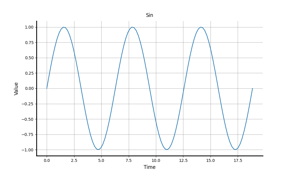
It’s very unlikely, however, that you will face such ideal waves with only one sine component at a time in the real world. Let’s now look at an example of an arbitrary sound wave that consists of many different frequencies and amplitudes.
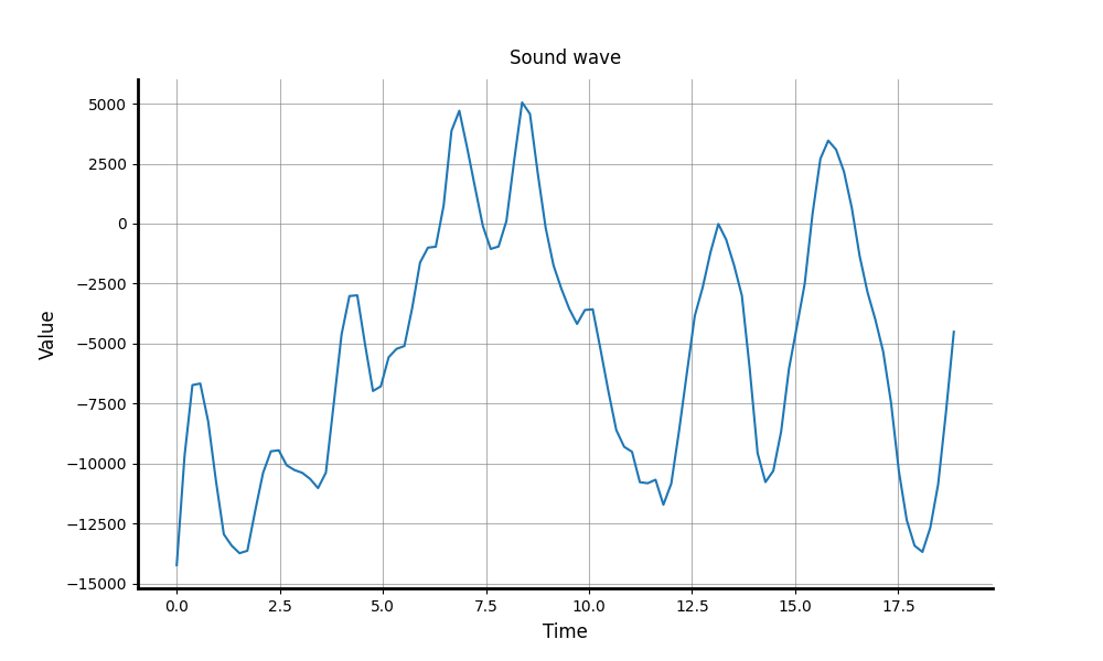
As you can see, it’s much harder to observe any pattern here. I should say that in this waveform many different frequencies coexist at the same time. Their sum gives the mentioned picture. The bass guitar, the drums, and the singer’s voice all occupy different frequency ranges, yet they exist within the same space.
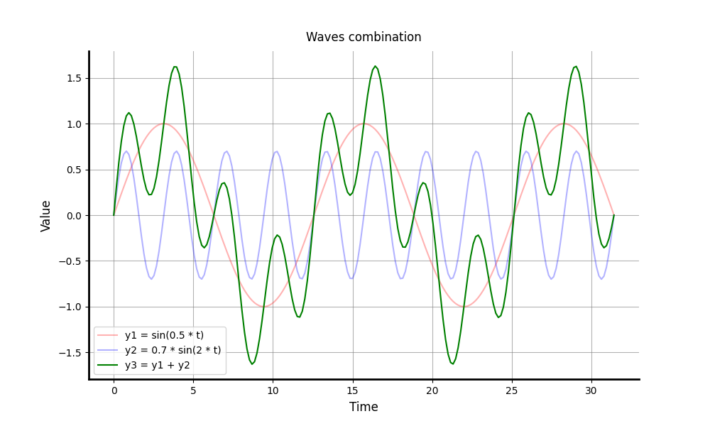
Looking at that complex waveform, it’s hard to observe any pattern. This is where the Fourier Transform comes in. It is a mathematical tool that allows us to decompose any complex wave into a sum of simple, perfect sine waves. Understanding that every sound is just a recipe of different frequencies is the foundation of modern audio processing, from equalizers to MP3 compression.
Discretization
I’ll give a piece of definition from Wikipedia first:
Discretization is the process of transferring continuous functions, models, variables, and equations into discrete counterparts. This process is usually carried out as a first step toward making them suitable for numerical evaluation and implementation on digital computers.
In the real world, sound is represented by continuous values, meaning data (amplitude of the wave at a given time for example) can take on any value within a given range. Between any two values, there is always another possible value (infinite decimal places).
Imagine a stone falling down from a steep hill; its motion is smooth, there are no discrete steps in the stone’s velocity or coordinate.
Values that are measured and can be broken down into smaller and smaller fractions are called continuous values.
On the other hand, discrete data consists of distinct, separate values. There are “gaps” between the points, meaning you cannot have a value in between two specific steps.
Computers are fully discrete machines, so in order to store and process the sound, we should first obtain its discrete form.
So, how do we do that? I’m going to explain the simplest method, called PCM (pulse code modulation). PCM is a method used to digitally represent analog signals. It is the standard form of digital audio in computers, compact discs, digital telephony and other digital audio applications. In a PCM stream, the amplitude of the analog signal is sampled at uniform intervals, and each sample is quantized to the nearest value within a range of digital steps.
To be precise: throughout this text, I use the term PCM to refer specifically to LPCM (Linear Pulse Code Modulation), meaning the sound is sampled at a fixed rate and the amplitude is measured using linear, equal intervals.
Sample rate
Imagine a microphone membrane moving together with some wave in the air. We cannot record the position of the membrane at all possible moments in time, but we can still record the position a fixed number of times per selected interval. For example: 8000 times per second, or 44100 times per second.
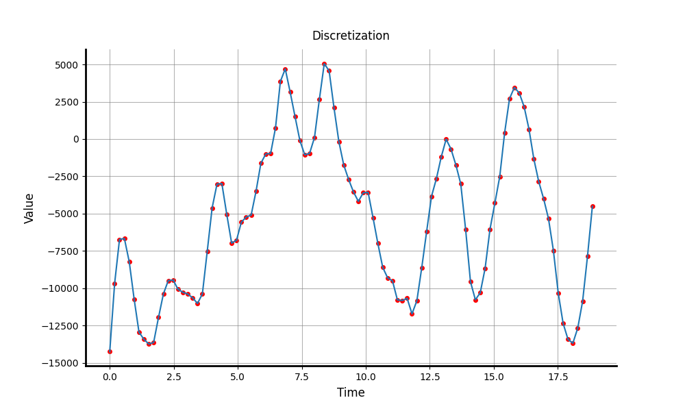
We record samples at a given rate (8 kHz, 44100 Hz, etc). This is the first characteristic of the discrete sound data - sample rate. This is also called “horizontal resolution”. It’ll become clear later why it is called horizontal and what vertical resolution is.
A bigger sample rate means we can record a sound wave more precisely and store more information. However, this leads to increased file sizes.
Important note
The Nyquist–Shannon sampling theorem states that to perfectly reconstruct a signal, it must be sampled at a rate greater than twice its highest frequency component. This threshold, known as the Nyquist rate, prevents aliasing by ensuring the discrete samples capture enough information to define the original continuous waveform.
For example, humans under normal conditions can recognize frequencies in the range between 20 Hz and ~20 kHz. So, in order to fully capture the sound perceived by humans, we should record sound at about 40 kHz rate.
Really, imagine if we record a high-frequency sound wave with some extremely low sample rate, let’s say a 1000 Hz sine wave recorded one time per second. Obviously, we won’t be able to correctly capture those high-frequency oscillations, we miss too much information.
Bit depth
Okay, now we record values with some fixed rate, but what kind of values do we record? Most of the time, we measure the wave’s amplitude and record it as some numerical value. For example, let’s say silence is represented as zero, and the loudest value is represented as 3 or -4 (there is no negative loudness, we just represent the values in a way that zero represents silence, and values farthest away from zero represent the maximum loudness).
So, we have a range: [-4, -3, -2, -1, 0, 1, 2, 3]
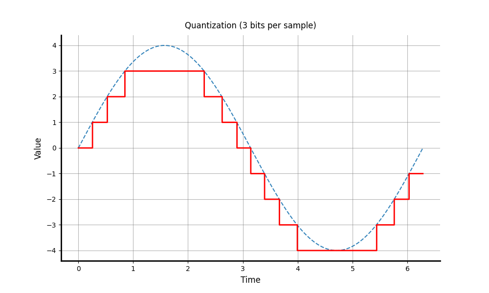
8 values, which can be represented by 3 bits (2 ** 3).
Our vertical resolution in this case is 3 bits. As you can see, the discrete form of the sine wave is very stepped, and the quantization error is pretty high (the difference between the real wave value and the quantized value).
This is another characteristic, and this is called “vertical resolution” or bit depth (how many bits of information a single sample carries).
Most of the time, we measure wave’s amplitude, and record it as some value.
For example: 8 bits, 16 bits, 24 bits or even 32 bits.
A higher bit depth reduces quantization error, which is the “rounding error” that happens when a continuous wave is forced into a fixed digital step. The higher bit depth - more possible values sample can take.
8-bit = 256 values. Retro games, telephony, lo-fi aesthetics.
16-bit = 65,536 values. CD Quality. Standard for most consumer audio.
24-bit = 16,777,216 values. Studio Recording. Provides "headroom" for editing.
32-bit (float) = Virtually infinite
Bitrate
It’s now enough information to define the bitrate of the sound data (how many bits per second). For example:
Music recorded at 8 kHz sample rate, 16-bit depth, and 2 channels (stereo) gives us 8000 * 16 * 2 = 256 kbps (uncompressed).
Encodings and containers
Generally speaking, PCM is the most fundamental way to encode analog sound into discrete digital values. Most PC sound cards require PCM-encoded data for playback. Because PCM maps directly to the wave’s amplitude, it is also the ideal format for audio editing and digital signal processing (DSP), such as applying filters or effects.
However, PCM is not the most efficient way to store audio. Because it records every single sample - even during silence - it results in very large file sizes. To solve this, we use various compression formats:
- FLAC is a lossless encoding of linear pulse-code modulation data
- MP3, AAC are lossy formats that remove “unnecessary” data. Often, developers of such codecs use the imperfections of the human ears
Those entities defined above are codecs (encoders/decoders) to manipulate binary data. However, how and where do we store this encoded data? Can encoded sound be interpreted without any additional information regarding its format? The answer is the following: we often need additional metadata (data that describes other data). Even for raw LPCM, the computer needs to know the Sample Rate, Bit Depth, and Number of Channels.
This is when the container comes in. These are the file formats that allow us to store sound data encoded with some codec, plus some additional information (such as which codec is used, the author’s name, text, and different characteristics of the sound.)
For example:
- WAV
- AIFF
- FLAC
- MP3 (used with MP3 codec)
- Ogg
Practice. WAV file format under the hood
Preparation
First of all, you need a WAV file with some arbitrary sound with LPCM-encoded data inside (16-bit depth will be used in the following example).
You can download some music or sound and convert it using Audacity or ffmpeg:
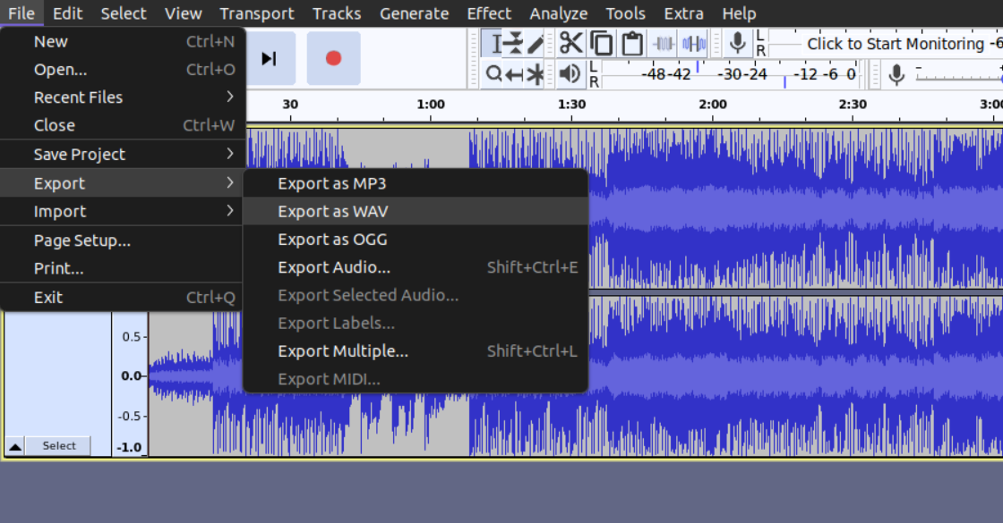
and then select the 16 bit signed PCM encoding
or
ffmpeg -i input_file -c:a pcm_s16le output.wav
WAV file structure
You can find a comprehensive WAV file format description here. In this tutorial, I’ll give some basic information needed to decode 16-bit PCM sound data.
In its basic form, a WAV file is a RIFF container file with the following structure:
| File Offset (bytes) | Field Name | Size (bytes) | Description |
|---|---|---|---|
| 0 | ChunkID | 4 | “RIFF” |
| 4 | ChunkSize | 4 | Size of entire file - 8 bytes |
| 8 | Format | 4 | “WAVE” |
| 12 | Subchunk1ID | 4 | “fmt “ |
| 16 | Subchunk1Size | 4 | 16 for PCM |
| 20 | AudioFormat | 2 | PCM = 1 |
| 22 | NumChannels | 2 | Mono = 1, Stereo = 2 |
| 24 | SampleRate | 4 | e.g., 44100 |
| 28 | ByteRate | 4 | SampleRate * NumChannels * BitsPerSample/8 |
| 32 | BlockAlign | 2 | NumChannels * BitsPerSample/8 (how many bytes per sample, considering number of channels) |
| 34 | BitsPerSample | 2 | e.g., 16 |
| 36 | Subchunk2ID | 4 | “data” |
| 40 | Subchunk2Size | 4 | Size of the raw sound data |
| 44 | Actual data | Subchunk2Size |
Decompose the file
Import the needed modules:
import struct
import subprocess

from collections import namedtuple
The struct module is a useful built-in Python module which allows you to unpack binary data into a structured format, following the format given as a parameter. For example:
- i - 4 bytes integer
- h - 2 bytes integer
- < - specify little endian order
- 4s - reads 4 bytes into bytes array of length 4
Open the file for reading in the binary mode:
wav_file = open('sound.wav', 'rb')
Let’s now read the first chunk and check its format:
riff_chunk_descriptor = wav_file.read(12)

riff_label, file_size, wav_format = struct.unpack('<4si4s', riff_chunk_descriptor)

print(f'Container name: {riff_label}')
print(f'File size - 8 bytes: {file_size}')
print(f'Container format: {wav_format}')
Get the characteristics of the sound:
WavFormatChunk = namedtuple('WavFormatChunk', [
    'FormatBlockID',   # 4 bytes: "fmt "
    'BlockSize',       # 4 bytes: Chunk size (usually 16)
    'AudioFormat',    # 2 bytes: 1 for PCM, 3 for Float
    'NbrChannels',    # 2 bytes: Number of channels
    'Frequency',      # 4 bytes: Sample rate (Hz)
    'BytePerSec',     # 4 bytes: (Frequency * BytePerBlock)
    'BytePerBlock',    # 2 bytes: (NbrChannels * BitsPerSample / 8)
    'BitsPerSample'   # 2 bytes: Bits per sample (e.g., 16, 24)
])

pcm_format_chunk = wav_file.read(24)

raw_tuple = struct.unpack('<4sihhiihh', pcm_format_chunk)
wav_format_chunk = WavFormatChunk(*raw_tuple)

assert wav_format_chunk.FormatBlockID == b'fmt '

print(
    f'PCM format chunk size: {wav_format_chunk.BlockSize}\n'
    f'Audio format: {"PCM" if wav_format_chunk.AudioFormat == 1 else wav_format_chunk.AudioFormat}\n'
    f'Number of channels: {wav_format_chunk.NbrChannels}\n'
    f'Sample rate: {wav_format_chunk.Frequency}\n'
    f'Bytes per sample: {wav_format_chunk.BytePerBlock}\n'
    f'Bytes per second: {wav_format_chunk.BytePerSec}\n'
    f'Bits per sample: {wav_format_chunk.BitsPerSample}\n'
)
Example output:
Audio format: PCM
Number of channels: 2
Sample rate: 44100
Bytes per sample: 4 # 2 bytes per sample (16 bit / 2) * 2 channels
Bytes per second: 176400
Bits per sample: 16
And now we are ready to extract the raw sound data from the file:
data_format_chunk = wav_file.read(8)

data_label, data_size = struct.unpack('<4si', data_format_chunk)

assert data_label == b'data'

print(f'Data size in bytes: {data_size}')

raw_data = wav_file.read() # Read the rest until the end of the file
At this point, I should explain what we have stored in our raw_data variable.
In our example, we have PCM encoded sound with 16 bits per sample, 44,100 samples per second, and two channels. I’ll illustrate it as follows:
      <byte1> <byte2>             <byte1> <byte2> ... and so on
 { Sample 1 | Left channel}  { Sample 2 | Right channel}
Let’s convert the first 10 samples into integers from raw bytes, just to see how this data looks like:
bytes_per_sample = wav_format_chunk.BitsPerSample // 8
bytes_count = bytes_per_sample * 10 * wav_format_chunk.NbrChannels # How many bytes we should read to obtain first 10 samples

decoded_10_samples = [int.from_bytes(raw_data[i : i + bytes_per_sample], byteorder='little', signed=True) for i in range(0, bytes_count, bytes_per_sample)]
Example output:
>>> decoded_10_samples
[0, 0, 0, 0, -1, 0, 2, 1, -2, -2, 2, 2, -3, -2, 3, 2, -3, -1, 4, 0]

Which means that first 10 samples represents almost complete silence

For signed 16-bit number we have range: [-32768 : 32767]
Finally, let’s pass our raw bytes directly to the sound card, without any headers or audio container formats to check if we have done our work correctly (I use aplay, a binary player for the ALSA sound card driver, which should be available on most Linux distributions):
process = subprocess.Popen(
    ['aplay', '-f', 'S16_LE', '-r', str(wav_format_chunk.Frequency), '-c', str(wav_format_chunk.NbrChannels), '-'],
    stdin=subprocess.PIPE
)

process.stdin.write(raw_data)
process.stdin.close()
process.wait()
Congratulations! I hope you were able to hear the sound or music you have chosen for this tutorial, and not some chaotic noise.
As you can see, there is no place for magic here. We were able to read sound data and its format following the set of simple rules described in the table above.
Grazie mille!